A machine learning model to understand fashion search queries
Our mission at Lyst is to help people find fashion that they want to buy. One of the main tools that we offer our users to browse our huge inventory is the search engine.
It is crucial that the results from our search engine are as relevant as
possible; our inventory is huge, we sell around 100,000 pairs of jeans
for example.
So we cannot maximise its potential unless we make it easy for our users to browse it.
Some search terminology
In real life
Imagine that you’re a salesperson at a bricks and mortar fashion retailer. Someone comes in and
asks you something like:
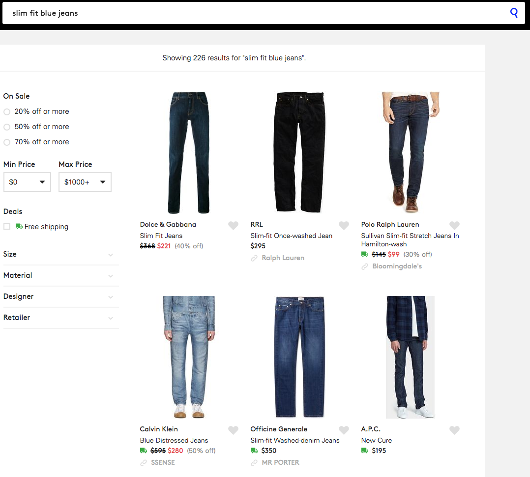
“Hi! I’m interested to buy some slim fit blue jeans, can you show me what you have?”
What happens next is going to look something like this:
- You are going to go around the shop and retrieve a selection of jeans that are relevant to what the user asked for.
- Then you’ll start showing them one by one to the customer, starting with the one that the client is the most likely to buy first.
In information retrieval
In information retrieval terms, those two steps are retrieval and ranking:
- You retrieve things which meet certain criteria.
- You sort them based on some score.
It’s important to note the criteria for retrieval is not binary (i.e. does the item match exactly or not), but continuous (i.e. it matches with a certain confidence.) If you’re looking for a blue t-shirt, some of them might be completely blue, but some of them might somewhere between blue and teal, some others might blue with white stripes. So you could rate how blue a given t-shirt is from 1 to 10 for example.
Back to real life again
To come back to our physical shop example, what if you have a very wide range of fits for jeans, and many different shades available? It’s not straightforward to decide what to pick, so you could proceed as follows:
- Trust your instinct and pick a selection of jeans which are “as blue and as slim as possible” (that’s what the user asked for after all)
- Now from that selection, the first jeans that you’ll try to sell to the customer are not always the bluest or slimmest jeans, but rather the ones that the user is most likely to buy.
Our previous search technology
Our previous search engine used the following two main pieces of technology:
- For retrieval: Elasticsearch, where we actually retrieve products based on text matching. For example if all the words in a user’s search query appear in the description of a product then it will stand a chance of being in the result.
- For ranking: A deep semantic similarity model.
In a nutshell:
- The model takes data about what products people click on in the context of a search result page.
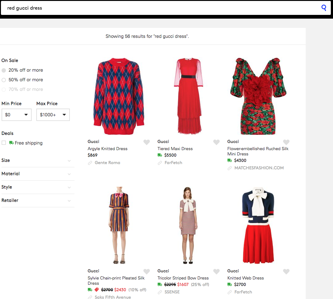
- So if a given dress is often clicked on for the search result page for “red gucci dress”, then that dress will move higher up for that search query.
Limits of the retrieval phase
For example a very popular designer these days is Off White.
- You can guess that simple string matching here will not get us very far here, as the products that we’ll retrieve will be a mixture of products that have white or off white in their descriptions (i.e. products which colour is white or off-white) rather than only products from the Off White designer.
- The thing that is missing here is that we’re looking for clothes belonging to the Off White designer.
We’ve been working lately on improving the retrieval part of the problem.
A 2-step approach for retrieval
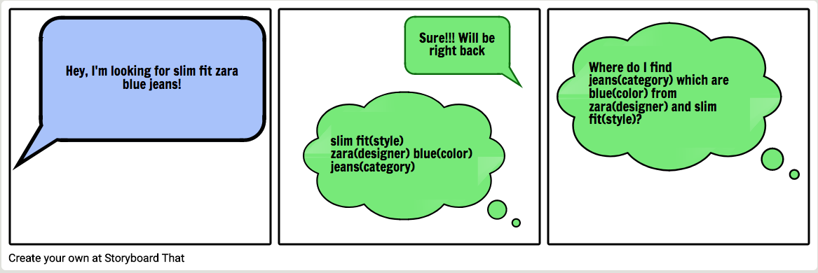
Let’s come back to the example of our physical shop again, here is an example of what the salesperson could think about what to do:
Retrieval Step 1: Entity recognition
Natural language processing jargon names this step entity recognition. The
task is to categorise the various words into various groups or classes.
In our case we focus on fashion_noun, designer, style, colour, material and gender.
For example we transform the unstructured search “red martin margiela sneakers” into a structured search of “colour: red, designed: martin margiela, category: sneakers”.
Retrieval Step 2: Entity linking
Once we have recognised the types of the words we need to map these to our actual products:
- Jeans is a category: where are the jeans in our shop? Oh they are under that denim sign.
- Blue is a colour: once I’ve found the jeans area, how do I determine which ones are blue? What if we have a very granular colour tagging in our shop, i.e. we have labels for dark blue, light blue, etc. Which ones do I pick? Only light blue and not dark blue? Is turquoise close enough?
- Slim fit is a style: We don’t have explicit fit labels on all the jeans, so do I know
which ones are actually slim fit?
Or we could have a situation where you have super slim fit and slim fit jeans in your shop, does the user mean both? Or only actual slim fit?
How it all fits together
Let’s come back to Lyst now. The approach that we’re trying to use is:
- When a user types in a search query, we’ll first try to categorise the various words in the text of the search query
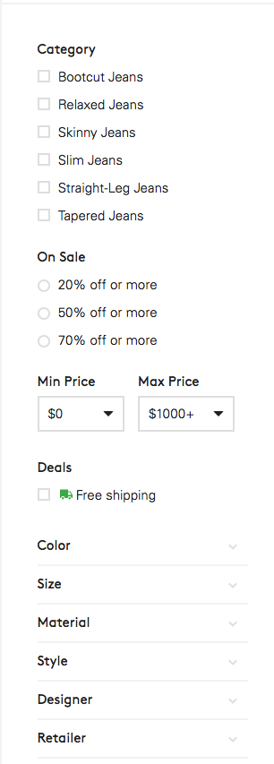
- Map the types of words we found in our search query to the product taxonomy seen below.
There are some potential limitations to this model here:
- What if we don’t understand everything the user says? What if the user uses words that won’t match the list of “types of words” that we’re considering?
- What if our taxonomy doesn’t capture everything that the user says? E.g. if the customer types in the actual reference number of a product, or the name of a specific model of a given product.
- What if it’s not straightforward to figure out what tags to consider once we understood what the
user says?
- Remember slim fit, what if we have super slim fit and slim fit?
- If someone asks for Hugo Boss clothes, does that also include Boss Orange and Boss Black?
The taxonomy has long been the central way all products on Lyst get organised. As a result our tags are quite consistent and we invest a lot on improving them. Using this data when possible is much better than relying on descriptions. For example if “jeans” appears in the description of a product, it might be a pair of jeans but it could refer to the material of a jacket.
An Entity Recognition model: Conditional Random Fields
We investigated two types of model to perform the first part of retrieval:
- Conditional Random Fields
- Long Short Term Memory neural networks
We’ve picked Conditional Random Fields (CRFs) over Long Short Term Memory Neural Networks (LSTMs), because LSTMs would have required much more up front work to get decent results (on our first try we used a bag of words). While the CRF model gave pretty decent results out of the box.
How it works in a nutshell
Conditional Random Fields are a class of models often used in machine learning as supervised models to classify elements of a sequence. The core idea is that they also look at neighbouring elements to decide what to predict.
Let’s start with a very concrete example, the model will have many feature functions that are like the ones below:
\[
f_1(y_t, y_{t-1}, sentence, t) =
\begin{cases}
10 \ \text{if} \ y_t = “designer”, sentence[t] = “offwhite” \
0 \ \text{otherwise}
\end{cases}
\]
\[
f_2(y_t, y_{t-1}, sentence, t) =
\begin{cases}
5 \ \text{if} \ y_t = “colour”, sentence[t] = “offwhite \
0 \ \text{otherwise}
\end{cases}
\]
Given a sentence, the model will return the classification that has the highest “score”, this score is basically the sum of all the feature functions, evaluated on all the tokens in the sentence:
\[ score(sentence) = \sum_{t=1}^{t=len(sentence)} \sum_{k}^{} f_k(y_t, y_{t-1}, sentence, t) \]
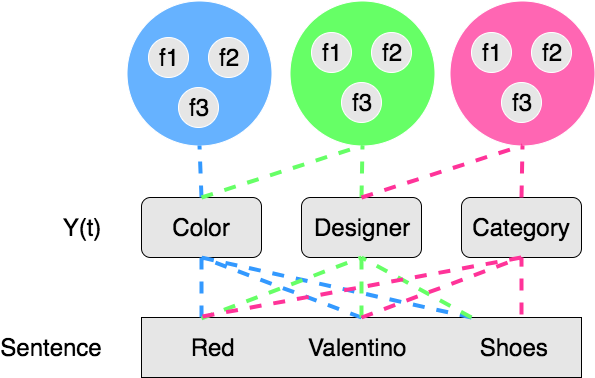
Note that every time we call a feature function, it will return a non-zero value only if the current and previous label (if any) \( y_t, y_{t-1} \) are equal to specific values. The sentence itself has to meet certain conditions.
The model defined by those feature functions will determine the best classification,
i.e. the \( (y_t) \) sequence that will maximise the score.
All those feature functions, the way they activate, their relative strength define how
the model will classify sentences.
And the training process consists of adjusting the weights in a way that fits
the training data as well as possible.
1/ A basic example
Consider the sentence “offwhite”:
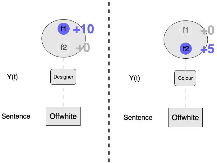
- if classified as \(offwhite(designer) \), then \( f_1 \) will give you 10 points and \( f_2 \) 0 points. Since \( f_2 \) deactivates if you didn’t choose “colour”.
- If classified as \(offwhite(colour) \), then you’ll get only the 5 points coming from \( f_2 \).
So given the feature functions we have, the model will classify the sentence as \( offwhite(designer) \)
The strengths of those feature functions (the values of 10 and 5) depend on the training set that we used to train the CRF model, if you have:
- a lot of \( “..offwhite(designer)..” \)
- not that many \( “..offwhite(colour)..” \)
Then the training process will detect that the token “offwhite” is more likely to be a designer than a colour. Hence f1 is “stronger” than f2.
2/ A more interesting example
Now let’s imagine where we have more feature functions, f3 and f4, such that our features
functions are:
\[
f_1(y_t, y_{t-1}, sentence, t) =
\begin{cases}
10 \ \text{if} \ y_t = “designer”, sentence[t] = “offwhite” \
0 \ \text{otherwise}
\end{cases}
\]
\[
f_2(y_t, y_{t-1}, sentence, t) =
\begin{cases}
5 \ \text{if} \ y_t = “colour”, sentence[t] = “offwhite \
0 \ \text{otherwise}
\end{cases}
\]
\[
f_3(y_t, y_{t-1}, sentence, t) =
\begin{cases}
30 \ \text{if} \ y_{t-1} = “designer”, y_{t} = “category”, sentence[t] = “tshirts” \
0 \ \text{otherwise}
\end{cases}
\]
\[
f_4(y_t, y_{t-1}, sentence, t) =
\begin{cases}
50 \ \text{if} \ y_{t-1} = “colour”, y_t = “category”, sentence[t] = “tshirts” \
0 \ \text{otherwise}
\end{cases}
\]
What do those feature functions mean?:
- f3 gives you 30 points if a classification looks like: “..(designer) tshirts(category)”
- f4 gives you 50 points if a classification looks like: “..(colour) tshirts(category)”
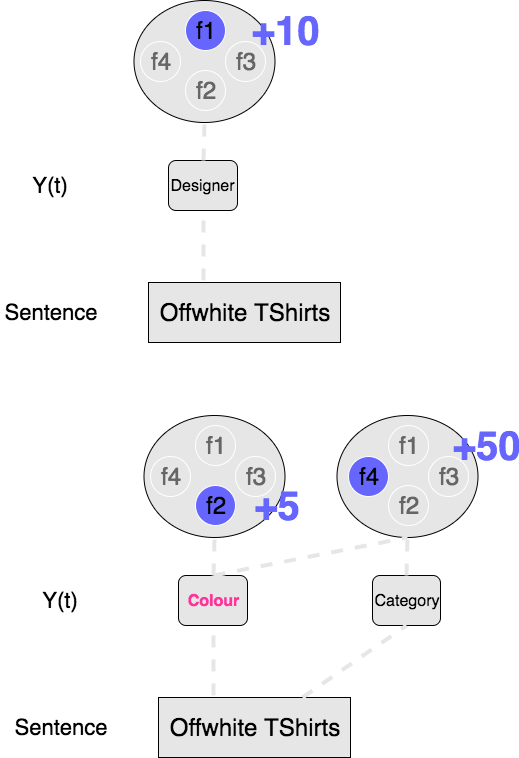
So now if the model has to classify the following sentence “offwhite tshirts”:
- Looking at the first token, you’d prefer designer as f1 beats f2. f3 and f4 need a previous token so they can’t run for the first token.
- Now if you move on to the second token, f4 is the most interesting feature function here as
it gives you 50 points. But in order for it to activate you have to:
- Classify “TShirts” as a category
- Classify the previous token “Offwhite” as a colour. As a result you’ll override your previous decision and activate f2 instead of f1. So you’ll lose points for the first token by changing your decision, but that loss will be offset by the important gains from f4 on the second token.
This could mean that the training set has:
- a lot of “offwhite(designer)”
- even more examples like “offwhite(colour) tshirts(category)”
We’ve now seen f1 and f4 “compete” against each other through their dependency on what is the class of the first token “offwhite”. The core ideas of the CRF model are:.
- Predictions for a given word depend on the predictions for neighbouring words
- As well as the value of the whole sentence
How we use the model in real life
You’ve surely noticed that the dependency on the value of the sentence is relatively simple,
conditions like: \( sentence[t] == token \).
Usually there’s many different feature functions that you can use, below are examples of the ones
that we use. Note that the condition can also look at the values of any other token in the
sentence.
Which is why the feature function receives the index to the “current” element but has access to the
whole sentence.
Also, in the examples above only one feature function was activated for a given word in the
sentence, but you can have more than one of course.
# The features below will be used to predict the label of word number i in the sentence
# sentence[i][0] the word itself, sentence[i][1] the POS tag
'word_length': lambda sentence[i]: str(len(sentence[i][0])),
'number_of_syllables': lambda sentence[i]: str(textstat.syllable_count(sentence[i][0]))
'low': lambda sentence[i]: sentence[i][0].lower(),
'title': lambda sentence[i]: str(sentence[i][0].istitle()),
'word2': lambda sentence[i]: sentence[i][0][-2:],
'prefix_word2': lambda sentence[i]: sentence[i][0][:2],
'pos': lambda sentence[i]: sentence[i][1],
'pos2': lambda sentence[i]: sentence[i][1][:2],
'upper': lambda sentence[i]: str(sentence[i][0].isupper()),
'digit': lambda sentence[i]: str(sentence[i][0].isdigit()),
'vowels_pct': lambda sentence[i]: str(_vowels_pct(sentence[i][0])),
'_contains_at_least_one_number': lambda sentence[i]: str(_contains_at_least_one_number(sentence[i][0])),
'colour_gaz': lambda sentence[i]: str(sentence[i][0].lower() in ENTITIES['colour']),
'material_gaz': lambda sentence[i]: str(sentence[i][0].lower() in ENTITIES['material']),
'gender_gaz': lambda sentence[i]: str(sentence[i][0].lower() in list(ENTITIES['gender'].keys())),
# Feature that depends on the previous word!!
'-1:word_length': lambda sentence[i-1]: str(len(sentence[i][0])),
...
# Feature that depends on the previous word!!
'-1:word_length': lambda sentence[i-1]: str(len(sentence[i][0])),
...
# Feature that depends on the next word!!
'+1:word_length': lambda sentence[i+1]: str(len(sentence[i][0])),
...
Each one of those “base features” will basically generate as many \( f_k \) feature functions as the number of values that they take (2 for booleans, the number of tokens you have for the identity function that we saw in the examples).
Entity Linking
So I’ve now explained how we go from there:
“red martin margiela sneakers”
to there:
“red(colour) martin margiela(designer) sneakers(category)”
We now need to map those recognised entities to actual values that can be applied to our filters.
Edit distance
The technique that we use at the moment is relatively straightforward, we use the edit distance metric, which is basically the number of key strokes that you need to type to go from A to B:
- “gucci” and “guci” have an edit(delete in this case) distance of 1
- similar with “gucci” and “goucci”
Basically as long as the token is not too different from one of our filter values, then those filter values will be selected.
And some aliases
However out of the box that’s not powerful enough. Let’s consider the designer called “maison martin margiela”. Users on our website usually spell it as:
- “maison martin margiela” or
- “maison margiela” or
- “margiela”
Edit distance doesn’t help us much here, given that in our database the canonical spelling is “maison martin margiela”, and “margiela” is quite far from that in terms of edit distance.
We basically decided to add all of the possible subsequences of a designer name (as long as that subsequence is specific to this designer alone) as an “alias” to it. So basically, if you search for “mmargiela”:
- mmargiela is recognised as “mmargiela(designer)”
- “mmargiela(designer)” matches “margiela” (the typo will be “corrected” if edit distance threshold is > 1)
- “margiela” (the alias) will apply the “maison martin margiela” filter
- You get to see the products that match the filter designer == “maison martin margiela”
More generally, for the various values of our filters we have synonyms to be able to capture all the variations of a specific filter value.
How well does it work?
This new search is currently deployed to 100% of our customers. We’ve seen an overall significant increase to our clickthrough rate, decrease in the proportion of empty search result pages, more conversion engagement etc. And we are actively investing in further improving the whole system (which is currently in its very first version).
It is quite interesting to note that we’ve witnessed pretty good results on our metrics despite only
about 20-30% of the search queries being fully recognised and linked.
When they’re not, we automatically fall back to the previous search engine technology.
Some numbers
Here are the classification accuracy metrics for the entity recognition phase (average of 5-KFold cross validation metrics):
| precision | recall | f1 | |
|---|---|---|---|
| designer | 0.784058 | 0.747632 | 0.765291 |
| fashion_noun | 0.900669 | 0.891801 | 0.896196 |
| material | 0.830343 | 0.767975 | 0.797396 |
| gender | 0.954635 | 0.977118 | 0.965650 |
| style | 0.726097 | 0.628055 | 0.672516 |
| colour | 0.891273 | 0.884205 | 0.887625 |
For entity linking, precision is nearly perfect given the very conservative 1 edit distance method.
Recall is quite tricky to analyse, if we fail to link a word it might be because of:
- a genuine inability of the linker to link to something that we have (genuinely bad recall). For example if someone asks for denim and we fail to link that to the jeans category
- the user asking for something that we actually don’t have in our inventory
This is still being investigated!
CRF Features importance
Here is a selection of some the features used by the model and their importance (produced by the excellent eli5 library. Note that we use the BILOU notation as entities can span multiple tokens.
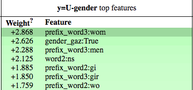
There’s only a handful of tokens that represent genders, here you can see that the model relies on:
word[:3] == "wom"(to capture “woman” or “women”)word[:2] == "gi"(to capture “girl”)- The gazetteer represents a hardcoded list of values that we passed to the model.
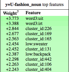
For fashion nouns, we depend on lot on clusters of fastText representation (more details below)
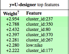
Similar for designers, notice the hardcoded value of “nike”!
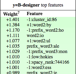
This one is quite interesting, should the following word be “by” (+1:word2:by), like in “adidas
by stella mccartney”, then this feature function will increase the odds that the current word is
the beginning of a designer entity!
The future
The areas that we’re going to explore to improve the quality of the whole system are:
- more hyperparameter optimisation (the model that we deployed to production was generated by a
very high level library that hardcodes most parameters to the low level python-crfsuite
library).
We will shortly switch to sklean-crfsuite that allows us to specify those parameters. - more feature engineering, in particular around fastText representations. We ran fastText on a corpus on product descriptions, clustered those and used the cluster ids for feature functions for the CRF model, those as the most important features for designer recognition.
- More annotation data (the training set that we used exclusively made of manual annotations), that could be artificially augmented (generating synthetic annotations based on existing ones)
- Investigating more complex models for entity linking, more synonyms for our value filters
- Supporting more entity types? (retailers, sizes etc.)
Thanks
Special thanks to everyone that has been involved in this project, including but not limited to:
- members of the data science team
- members of the seek squad
- members of the copy team (who spent long hours annotating thousands of search queries so that we could train the model)
