Color Detection

At Lyst, we process millions of fashion products a day from over 500 retailers. One of the goals of the data-team is to transform this stream of semi-structured data into one consistent product catalogue. Colour is one of the most difficult fields to normalise. For example here are a selection of colors we saw in the past week.

Image	Retailer Color	Actual Color
	Orchid Placement	Blue & Pink
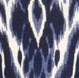	Australian Tribal Ikat	Blue & White
	High Voltage Melange	Pink
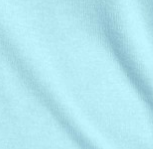	Deep Misty Fjord	Blue
	From Russian With Love	Grey

Some of these colors can be deciphered by a human but all are very difficult for a computer. Even simple colors such as snakeskin or periwinkle can be hard to process automatically. In the past, we used a range of techniques to map retailer colors to lyst colors, from simple keyword matching to complex ML models. We found that these methods produced unsatisfactory results due to complexity of color names used by retailers. The only way we’ve found to accurately determine product color is via the product images.

Color clustering

To find the colors of an image we use clustering on an Nx3 matrix where each row of the matrix represents an RGB pixel. The main colors of an image are deemed to be the cluster centers. Our use of clustering was inspired by this article from Charles Leifer. Instead of using a fixed cluster size, we used an algorithm that dynamically determine the number of clusters (see mean-shift or DBSCAN in sklearn) because a fixed number of clusters tended to result in muddy colors.

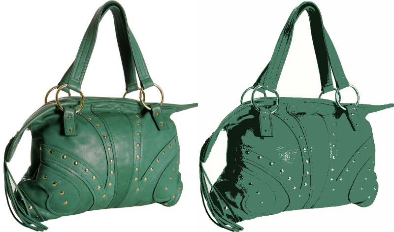
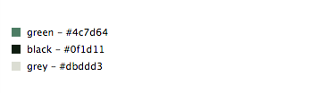
The images below demonstrate how well this technique works. The first image shows the detected colors ordered by the percentage of pixels in their respective cluster. Even the dots of color in the t-shirt were detected. The second image shows the cluster-space pallet. You can see that shadows have been clustered with green whilst highlights have been clustered with pink.

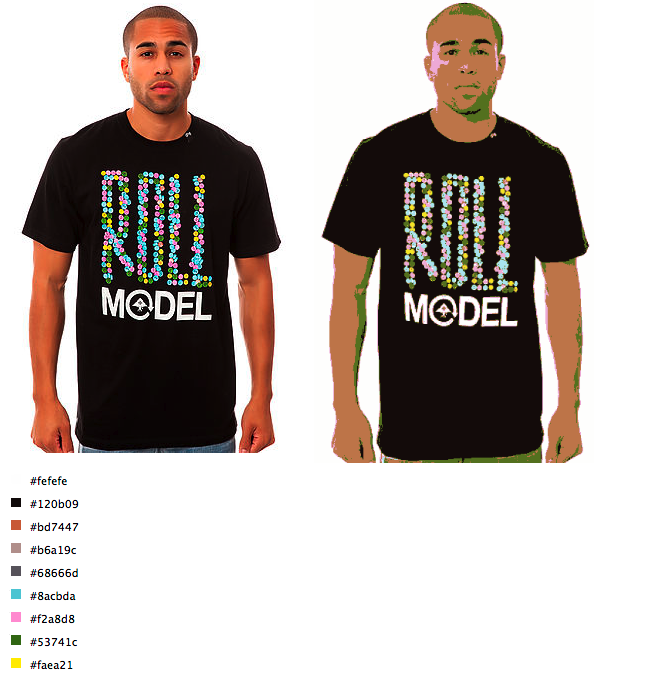
One major issue is that the first color is almost always going to be the background. My colleague Carl has a blog post on how we remove backgrounds. When used with this clustering technique, we can even detect colors on images with graduated backgrounds.

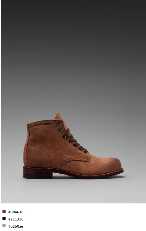
Now we can extract accurate hex colors for the majority of our product images. The next step is to translate these hex values into color names.

Color names

At Lyst we use a small set of color names to describe products. These names are stored internally and used on the website so that users can filter by color.

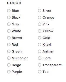
Mapping from a hex value to a color name is more complex than it seems; for instance, when is a red considered pink or when does grey become black. The solution to this problem came from Randall Munroe of xkcd fame and his Color Survey.

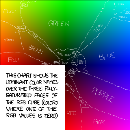
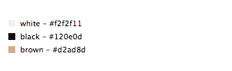
The survey consisted of asking his readers to identify hex colors by name. The result is a list of 200k RGB values and names for those colors picked from a small set. The mappings required some changes to fit into our color system because we need extra colors such as beige and grey. We also added hardcoded thresholds for white and black as it is almost impossible to have perfectly white and black clothes in images.

With 200k entries the mapping is not complete over the RGB space (200000 / 255^3 is around 1.2%) so to map all hex colors to names we need to consider the distances between colors.

Color distance

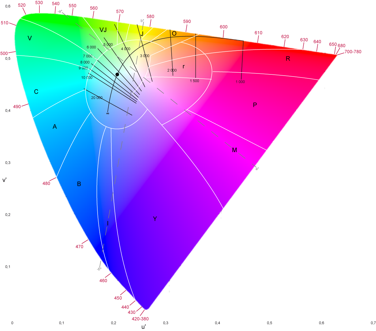
The data from xkcd is not complete so we need some way of finding similar colors. To define a metric of color difference we first need a space in which to measure distance. The RGB space is not suited to measuring color difference because distance magnitudes in the color space do not necessarily correspond to the magnitude of color difference as perceived by humans. To rectify this deficiency the International Commission on Illumination (CIE) defined the Lab color space which aims to attain so called perceptual uniformity.

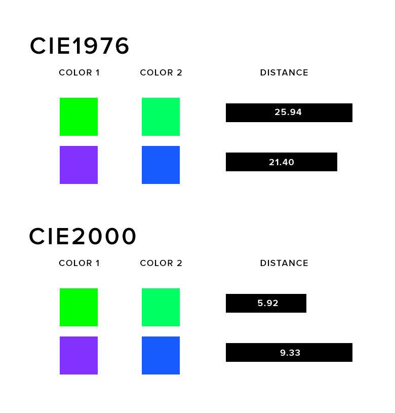
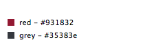
CIE has defined a number of color difference functions. The simplest being CIE1976 which is euclidean distance on the Lab colorspace. The latest, CIE2000, attempts to rectify issues that CIE1976 has with perceptual uniformity as shown in the figure below. Under CIE1976, the two shades of green are considered further apart than blue and purple but under CIE2000 this is no longer a problem (thanks to Rok Carl for the image).

Now that we have a measure of distance the issues becomes: give a color C how do we find the nearest color in the xkcd matrix? The xkcd matrix consists nearly 200k colors so we would have to calculated CIE2000 200k times whenever we wanted to name an color. This process is extremely expensive. On a 2013 macbook finding one color name takes over 5 seconds.

To speed up the color difference calculations we decided to vectorised deltaE. The standard deltaE functions are already implemented in the colormath python package. We ported these to numpy and added a function to take a numpy array of Lab coordinates. When used with large data-sets the vectorised implementation is 25-180 times faster depending on which distance function is used. The vectorised delta E functions are now available in the colormath package and can be used in the following manner.

import csv
import numpy as np

from colormath.color_objects import LabColor

# load list of 1000 random colors from the XKCD color chart
reader = csv.DictReader('lab_matrix.csv)
lab_matrix = np.array([map(float, row.values()) for row in reader])

# the reference color
color = LabColor(lab_l=69.34,lab_a=-0.88,lab_b=-52.57)

# find the closest match to `color` in `lab_matrix`
delta = color.delta_e_matrix(lab_matrix)
nearest_color = lab_matrix[np.argmin(delta)]

print '%s is closest to %s' % (color, nearest_color)

Results

Now we can quickly deduce the hex color and color name of a product from its image with a high-degree of accuracy.

Currently these colors get sent to humans to moderate (they can do this quickly thanks to a powerful interface), but in the future we hope to improve on these technique and completely automate color detection. A couple of Interesting future improvement would be to account for locality in the clustering and to use deltaE as the clustering distance function.