Working with Fashion Models

Being a fashion company we often have to work with temperamental high-maintenance models, by which (of course) I mean machine learning models.

Fashion is a visual medium so it makes sense for our models of fashion to include visual features. One typical use-case at Lyst is ordering a set of products in accordance with some critera. Most retailers use human experts to order products manually (so called ‘merchandising’) but Lyst has so many new products a day that this process must be automated and personalised for each user.

We hypothesize that when a user browses products they primarily make visual judgements based on the images rather than based on the textual description. If we order the products using only textual features then it will be hard to match user expectations and replicate the manual merchandising process. – to do this we need image feature

Our task has some special requirements.

• representation: much of the ML infrastructure at lyst is based around quickly searching for similar vectors (i.e. duplicate detection, product search and recommendations). So ideally we would use a method that produced a representation. Once learnt, the representation could also be used as the input for other models without having to process all the images again.

• multi-image: fashion products, for the most part, have multiple images so our model should be able to map these down to one product representation. Previously we have use models with single image inputs and aggregated the results (i.e. mean or sum) but it would be better to do this in a supervised manner.

• multi-task: We have multiple labels for each of our products (e.g. color and gender) and we want to use all of this information in our visual model to learn an optimal representation that can be used for many applications.

Given our above requirements, a convolutional neural network (CNN) is the obvious model choice. I won’t discuss how CNNs work as there are many other articles written by more knowledgeable people that already do an amazing job (here, here and here for example).

The Data

Before diving into the model, let’s talk about our data. The main data citizen at Lyst is the product. A product is a fashion item that’s buyable from 1 or more retailers. Each retailer has its own textual description and images for the product.

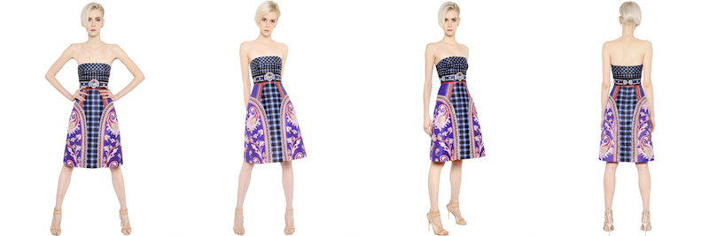
Below you can see that our images exhibit variation in terms of scale, alignment and orientation. They can also have variation in lighting and background.

Product are tagged with meta-data by our moderation team, 5 of which we will be using as labels to train our model; gender, colour, type, category and subcategory. Gender is male or female, colour is one of our 16 “Lyst colours”. Type, category and subcategory form our internal fashion taxonomy. Examples include shoes -> trainers -> hi-top trainers and clothing -> dresses -> gowns. There are only 5 types but 158 subcategories.

The Model

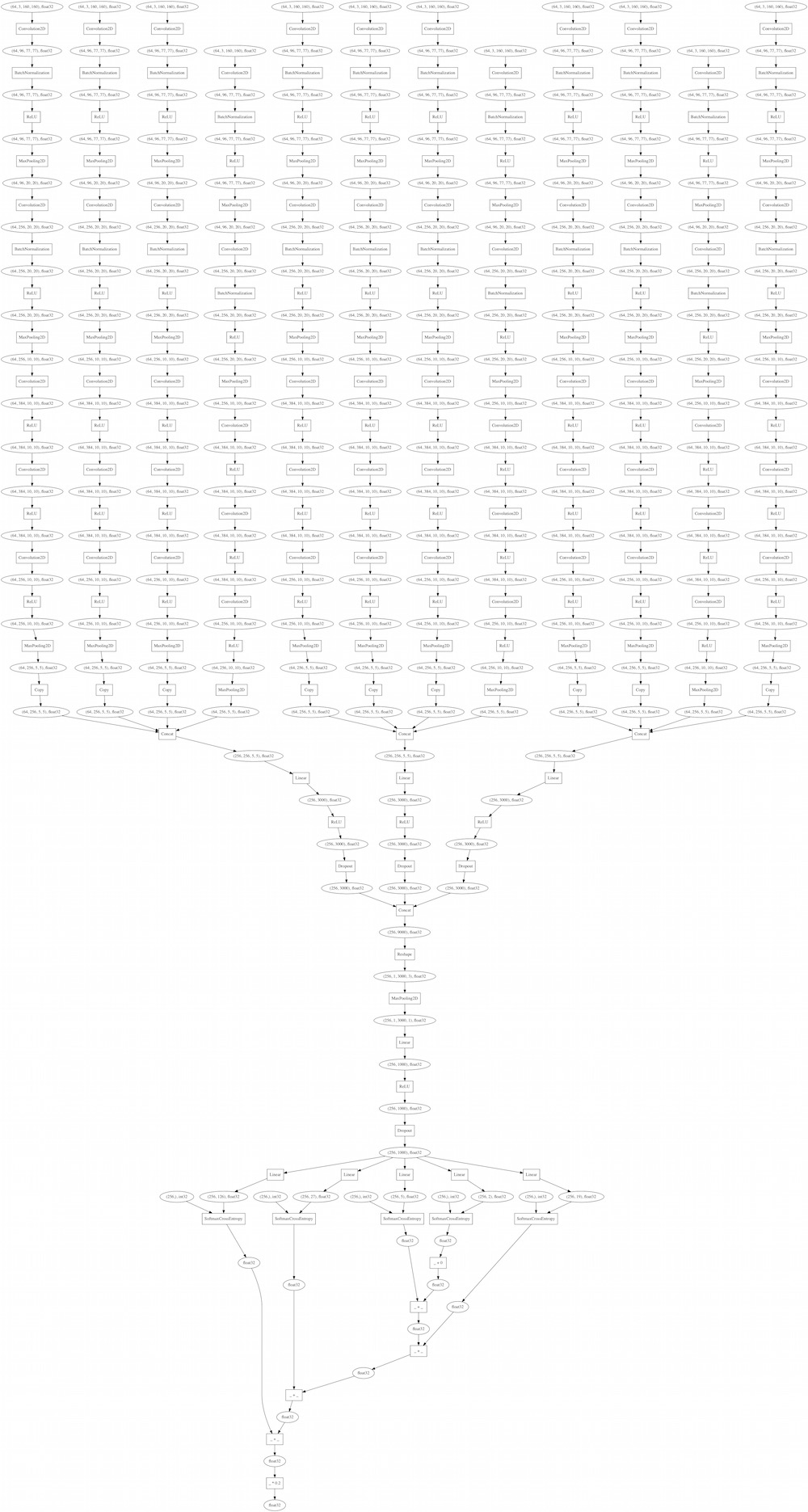
See below for a high-level overview of our network architecture.

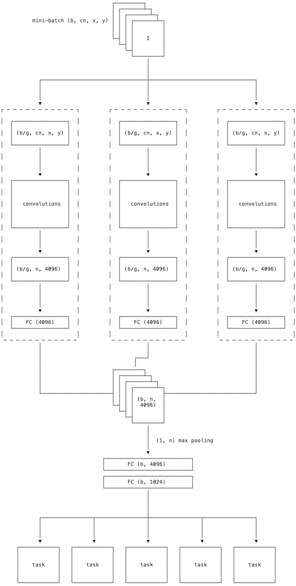
The input to the model is a tensor of dimensions (b, c * n, x, y) where:

• x and y are the image dimensions (usually x = y and in this case x = y = 224)
• c is the channels of the image (usually c = 3 for colour images)
• n is the number of images per product for the batch where 0 < n < 6
• b is the batch size or number of products per batch

This gives us b * n images per batch. Each batch is distributed among g GPUs so it must hold that b % g == 0. The distributed batches are processed by the convolution layers in parallel (data parallelism). The convolution params are shared between GPUs. The master params are copied to each gpu at the beginning of each mini-batch but the backprop updates are only applied to the master params. The convolutional architecture is based on ZFNet (an improvement on alexnet with smaller initial filters). This choice was due to the limited hardware we had at the time. We’ve since upgraded our GPU infrastructure and now we are using more modern architectures.

After convolution we have b * n representations of length 4096 (one per image). Each representation is passed through a dense layer (the pre-pooling layer) and then all image representations for a given product are column max pooled (i.e. n x 1 pooling) to give a single representation for each product. The intuition behind column pooling is: if one image strongly activates for a particular feature, then the pooled representation should contain that strong activation.

This aggregated representation is then passed through 2 more dense layers (the post-pooling layers) to give us a (b, 1024) matrix of product representations. The representations are then used to predict the 5 tasks. The losses of these tasks are average with the hope that the representation will be optimised for all 5 tasks.

Training

In terms of pre-processing we use the semi-standard method of mean subtraction with an aspect-ratio preserving scale followed by a random crop. For regularisation we randomly copy and mirror half the batch horizonally. We do not use other augmentations like rotation or vertical reflection because the objects in our images are rarely, if ever, angled in that manner.

We used chainer for training. You can view the computational graph of a typical mini-batch here). We trained on AWS using 4 GPUs. The model is trained via SGD with momentum and the learning rate was controlled manually based on the validation set loss. We used batch normalisation with dropout and weight decay. With the ZFNet architecture, we had to use a batch size to 64 due to hardware limitations. We trained for 20 epochs and dropped the learning rate by an order of magnitude twice from the initial value of 0.01. We found this produced better results than using an adaptive learning rate based algorithm.

The Results

We ended up with a global accuracy of 73% on the validation set.

	Multi-task	Gender	Color	Type	Category	Subcategory
Accuracy	0.731	0.886	0.675	0.947	0.661	0.485

Some tasks were are easy (type @ 95%), other tasks such as category were much harder. The multi-task accuracy can be boosted above 80% with the inclusion of textual features and we recently boosted colour accuracy over 90% by fixing our labels.

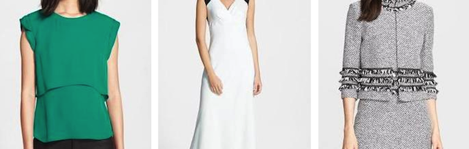
Misclassifications

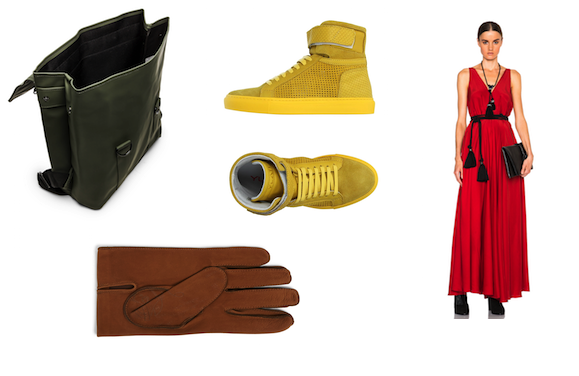
Below are some randomly sampled misclassifications for the color task to give an idea of where the model struggles. A number of decisions the model makes with regards to color are obviously wrong. Here it predicts the three items to be pink, black and blue respectively.

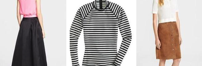
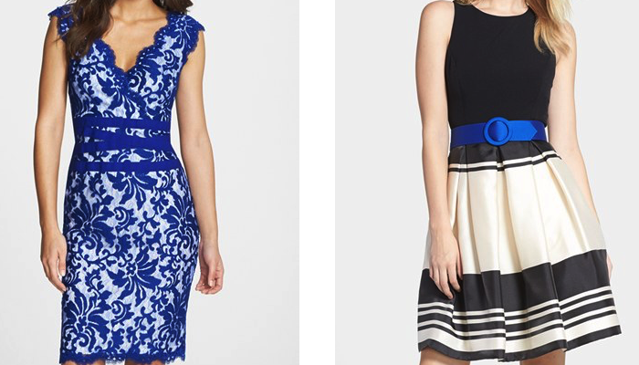
The model can fail when multiple colors are promient in the image. The model predicts black for the first image (pink is correct) and brown for the final image (white is correct). This may be one of the reasons that including text boosts the model’s accuracy; the text disambiguate images containing multiple products. The second image was predicted as black but tagged as white, both are correct but we do not currently account for multiple colour labels.

Finally, it can fail when the choice of color is ambigious or the human moderator has labelled the image incorrectly.

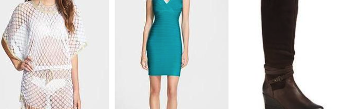
The first image was labelled as white but predicted as pink due to the flesh tones. The second image was labelled as blue but predicted as green when in fact it should probably be teal but we don’t have a teal color label. The last image was wrongly labelled as black and the model predicted the colour correctly as brown.

For other tasks, such as category, we see similar patterns of failure around ambiguity.

The first was predicted as nightwear but labelled as a dress; the second was predicted as a top but labelled as a dress.

Internals

Unlike regression or decision trees, neural networks cannot be easily interpreted via the parameters. Instead we have to use the input and output of the model to infer what is happening inside. The exception to this is the initial layer of weights. The initial filter layer operates directly on the input so the depth of the filters is the same as the number of image channels, as such we can treat the filters as RGB images.

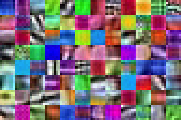
The filters look to be a combination of color detector and edge detectors with a stronger emphasis on colour than traditional imagenet models. Below are the filters for a model trained on colour only and with the initial layer having only 1x1 filters.

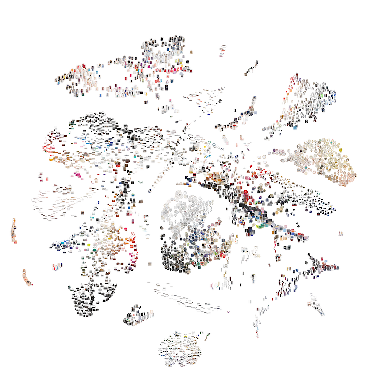
To give an idea of what the model is learning over all tasks, we’ve mapped the multi-task representation down to two dimensions using t-SNE and plotted the results.

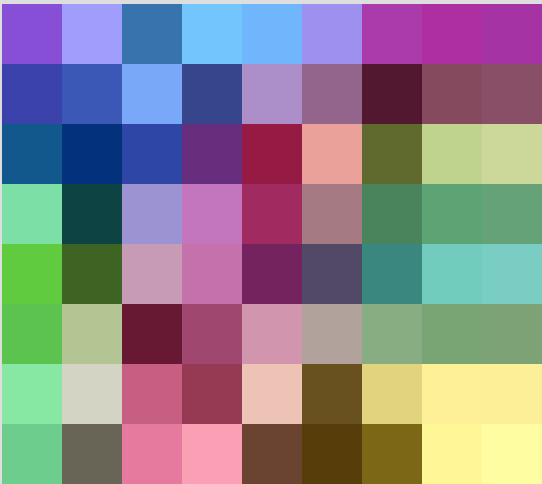
We can do the same with a model trained purely on the color objective whereby each point represents an item of clothing of that colour

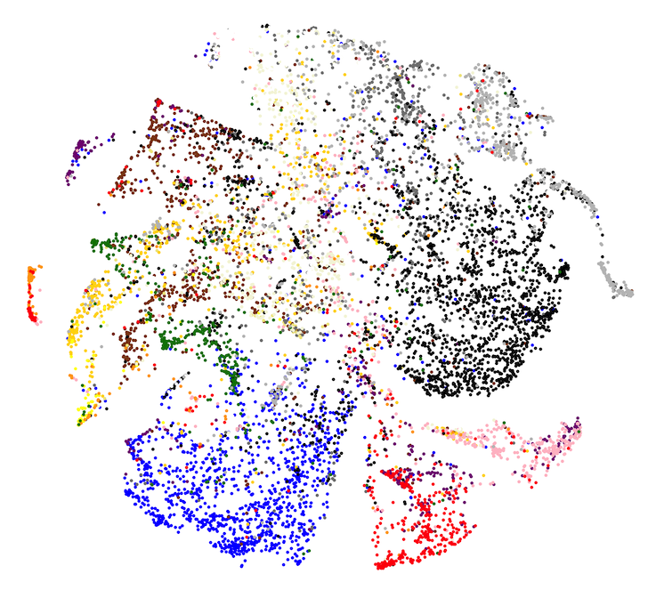
In the above plot we can see some interesting details about the ambiguity of colour names, similar to what we saw in the colour misclassifications. The orange-red cluster off to the left could represent coral (we currently do not have a coral color label). The mix of green, yellow and brown, I suspect, indicates a confusion over tan, khaki, beige and such.

Multi-task & multi-image

In terms of classification accuracy, the hope behind multi-task learning is that what is learned about one task can be applied to the other tasks such that each individual task performs better in a multi-task settings than they would in a single-task settings.

The table below show multi-task accuracy vs single-task accuracy for two of the harder tasks, category and colour. The network architecture and training scheme were kept identical, the only difference being the number of epochs and the learning rate schedule which was selected for each task to give the best accuracy.

	Color	Category
Multi-task	0.675	0.661
Single-task	0.678	0.662

The performance of the two models is very similar. So in this case there may not be much shared knowledge between tasks but I think we’ll see benefits when the representation is used in other applications (such as our search or recommendation algorithms).

To see if using multiple images is beneficial we will train a equivilent single image model. Although the main advantage for us of the multi-image model is that we can have one representation for a product rather than one for each image. We flatten the image groups so instead of have 1 product with n images, we end up with n copies of a products with 1 distinct image each. In this manner we have the same training data but can see if multi-image training helps or not. Again, architecture and training scheme were kept identical.

	Multi-task	Gender	Color	Type	Category	Subcategory
Single-image	0.703	0.856	0.656	0.930	0.633	0.442
Multi-image	0.731	0.886	0.675	0.947	0.661	0.485

Multi-image outperforms single-image across every task.

Conclusions

Using a simple off-the-shelf CNN we’ve quickly created a bespoke solution tailored to our data. For me, the power of deep learning is the ability to slot together components like lego. The model was developed in 2016 and as of today, we are using this representation for colour classification, duplicate detection and NLP tag extraction.

For more details see the following Lyst pydata presentations:

• Eddie Bell (YouTube, slides).
• Calvin Giles (YouTube, slides).